Inference: From noise to words

This is Part 1 of our Inference Engineering series. Read the other articles: Part 2: Making every denoising pass fast · Part 3: Fewer, smaller forwards.

Text diffusion (generating text by gradually reversing noise or corruption) did not begin as a faster way to run a language model. It began with a more basic question: can a model generate discrete symbols by reversing corruption, even though language is ordered, categorical (drawn from a fixed set of labels), and unforgiving of small mistakes?

Autoregressive (left-to-right, one-token-at-a-time) language models generate by extending a prefix one token (a vocabulary unit such as a word piece) at a time. The factorization is exact and familiar:

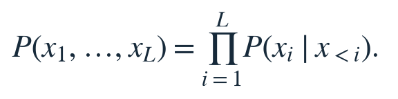
It also creates a chain that hardware cannot parallelise across time. Token i+1 cannot be computed until token i has been selected. A GPU (graphics processing unit) may contain thousands of arithmetic units, but a single sequence still advances through one dependent decoding step after another.

Diffusion offers a different shape of computation. Corrupt many positions, then train a model to reconstruct them together. During generation, refine a whole set of uncertain positions in parallel. The idea is simple: replace a long chain of one-token steps with a shorter sequence of wide denoising passes (model forwards that clean many positions at once).

For text, that idea was not enough on its own. Each of the next sections is a constraint that had to be solved before wide denoising could look like a real language-model runtime.

Constraint 1: text is not a small image

Image diffusion usually works in a continuous space (real-valued vectors rather than discrete labels). Add a little Gaussian noise (random noise from a normal distribution) to a pixel or latent vector (a compressed continuous representation) and the result is still a valid real-valued tensor (multi-dimensional array). The model learns to reverse many small perturbations.

A token has no comparable notion of a small numerical displacement. Changing cat to car is not a tiny move in vocabulary index space. Token IDs are names, not coordinates. Language also has sharp structural dependencies: one changed brace can invalidate a program, and one changed negation can reverse a claim.

Early text diffusion therefore split into two broad approaches. The first moved text into a continuous embedding space (learned real-valued vectors for tokens) and diffused there. The second kept the process discrete and defined corruption directly over categorical token states. Both could generate language. The discrete branch is the one that later carried the main line of token-level diffusion.

Constraint 2: corruption needs a native discrete process

In 2021, Hoogeboom and colleagues introduced multinomial diffusion (diffusion over category labels) for categorical data. Instead of adding Gaussian noise, the forward process (the noising process) gradually replaces a category with samples from a uniform categorical distribution (every vocabulary item equally likely). For a one-hot token (a vector that is 1 for the true class and 0 elsewhere) xₜ₋₁ in a vocabulary of size K,

Here Cat means a categorical distribution. The parameter βₜ controls how much information is destroyed at step t. Repeated application gives a closed-form distribution at any time:

As t grows, the sample remembers less about x₀ and approaches a simple noise distribution. A learned reverse model (the denoiser) then tries to recover the clean category. That answered the first hard question: diffusion can live on categories without pretending tokens are coordinates.

What remained open was flexibility. Multinomial diffusion gave one useful corruption recipe. It did not yet say which other corruption processes might train better, or how the process should connect to the masked prediction (predicting hidden tokens from context) already used in language models.

Constraint 3: corruption has to become a modelling choice

Austin and colleagues generalised the construction later in 2021 with Discrete Denoising Diffusion Probabilistic Models, usually shortened to D3PM (a family of diffusion models with discrete transition matrices). Their central object is a transition matrix Qₜ (the matrix that maps one categorical distribution into the next):

Changing Qₜ changes the meaning of corruption. It can send tokens toward a uniform distribution, favour semantically nearby categories, or move probability into an absorbing state (a sink that once entered is never left) such as [MASK] (a special blank token). Corruption stopped being a fixed recipe and became a modelling decision.

The absorbing construction also exposed a useful connection. If clean tokens are progressively replaced by a mask and the model predicts the originals, the training signal begins to resemble masked language modelling. Under particular schedules, D3PM relates BERT-style (Bidirectional Encoder Representations from Transformers) denoising and autoregressive cross-entropy (a standard next-token training loss) to the same probabilistic framework. Masked prediction was no longer only a representation-learning objective. It could define a generative reverse process.

The field now had discrete state spaces and selectable corruption. Two gaps remained: some groups still preferred continuous embeddings for control, and discrete reverse learning still needed stronger objectives before quality could approach autoregressive models.

A useful side branch: continuous embeddings for control

Diffusion-LM (a continuous-embedding text diffusion model), introduced by Li and colleagues in 2022, took the continuous route. It mapped tokens into continuous embeddings, applied Gaussian diffusion, then rounded the final vectors back to words. Its main focus was controllable generation: attributes could guide the reverse trajectory without retraining the base generator.

That solved a real problem, control without fine-tuning the whole generator, by accepting a different state space. Rounding embeddings back to vocabulary items works for some applications, but it also reintroduces a discrete recovery step after a continuous trajectory. The later discrete line kept tokens as categories throughout, which made training and sampling look more like ordinary language modelling.

“Text diffusion” therefore names a family of ideas, not one uninterrupted implementation lineage.

Meanwhile, back on the discrete side, Campbell and colleagues supplied a continuous-time Markov-chain (CTMC: a process that jumps between discrete states in continuous time) formulation in 2022. That framework underlies continuous-time CTMC methods such as SEDD (Score Entropy Discrete Diffusion). MDLM (Masked Diffusion Language Models) also uses a continuous-time objective, but derives its masked formulation without requiring CTMC theory.

Constraint 4: discrete reverse learning needed better objectives

By 2023 and 2024, discrete diffusion worked, but autoregressive models still set the practical standard for likelihood (how well the model assigns probability to text), scaling, and generation quality. The next bottleneck was the learning signal itself.

Score Entropy Discrete Diffusion, or SEDD (a discrete diffusion method that learns probability ratios between states), changed how the reverse process was learned. Rather than directly predicting a conventional continuous score, SEDD estimates ratios between probabilities of discrete states. For a state x and any alternate state y≠ x, its concrete score has the form

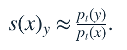
Lou and colleagues paired those ratios with a score-entropy objective and reported competitive GPT-2-scale (OpenAI’s smaller generative language model family) language modelling results. The contribution was not merely another corruption schedule. It supplied a discrete counterpart to score matching (learning the gradient of the log-density) that respected the categorical state space.

Masked Diffusion Language Models, or MDLM (absorbing diffusion trained with a masked-token loss), took a different route. Sahoo and colleagues showed that absorbing diffusion becomes surprisingly simple with the right parameterisation and estimator. For one token, the forward distribution can be written

where m is the mask state. The resulting continuous-time objective reduces to a weighted masked-token cross-entropy. Already visible tokens are carried through, while the model predicts only corrupted positions.

Ou and colleagues showed through Reparameterized Absorbing Discrete Diffusion, or RADD (a reparameterisation that links absorbing diffusion to clean-data conditionals), why this simplification is possible: the relevant reverse ratios can be expressed through conditional predictions of the clean data multiplied by an analytic time-dependent term. Together, these results made masked diffusion look less like an exotic alternative to language modelling and more like a generative extension of familiar masked prediction.

The training story was now coherent enough to ask the next question at full model scale.

Constraint 5: the model has to get large without losing the point

Nie and colleagues scaled masked diffusion models to 1.1B (1.1 billion) parameters, and LLaDA (Large Language Diffusion Models) later trained an 8B masked diffusion language model from scratch with pretraining and supervised fine-tuning (SFT: training on instruction or demonstration data after pretraining). LLaDA showed that a bidirectional denoiser (a model that attends to both left and right context) could acquire many capabilities associated with large language models.

Size alone, however, exposed a structural awkwardness. A full-sequence diffusion model wants to know the output length in advance. Long generation also makes every denoising pass wider. A model that refines an entire response at once gains parallelism, but it loses the flexible left-to-right extension that makes autoregressive generation convenient.

So the research had solved discreteness, flexible corruption, and better objectives, then proved that denoisers could be large. What it still lacked was a generation schedule that could grow without fixing the whole response length up front.

Constraint 6: long generation needs blocks and a cache

Block generation provides an interpolation. Split a sequence into blocks x⁽¹⁾,…,x^(B). Generate the blocks from left to right, but denoise positions within the current block in parallel:

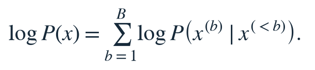
With a block size of one, this approaches ordinary autoregression. With one block covering the sequence, it approaches full-sequence diffusion.

SSD-LM (Semi-autoregressive Simplex-based Diffusion Language Model) explored an early semi-autoregressive block design in a continuous vocabulary simplex (a probability vector over the vocabulary). Block Diffusion, introduced by Arriola and colleagues in 2025, formalised a discrete version that is autoregressive across blocks and masked-diffusive within each block. It also used KV caching (reusing stored attention keys and values for finished tokens) across completed blocks, making arbitrary-length generation practical.

Block schedules and KV caching made long, flexible generation practical. A large open model could keep the parallel work inside a block while still extending text indefinitely.

Google’s public material does not present a paper-by-paper dependency through Block Diffusion or LLaDA, and the corruption process below is different. Treat the earlier papers as the constraints they removed, not as undocumented internals of the model that follows.

DiffusionGemma

Google DeepMind released DiffusionGemma (an open text-diffusion model built on Gemma) in June 2026 as an experimental open-weights model. It is fine-tuned from the Gemma 4 26B A4B Mixture-of-Experts architecture (about 26 billion total parameters with roughly 4 billion active per token). The published specification lists 25.2B total text parameters, 3.8B active parameters, 30 transformer layers (stacked attention and feed-forward blocks), a 262K vocabulary, and up to 256K tokens of context. Each MoE layer routes a token to 8 experts (specialised feed-forward networks) from a pool of 128, plus one always-active shared expert.

The design maps onto the constraints above in a fairly direct way.

Uncertain positions stay discrete vocabulary tokens. There is no continuous embedding trajectory that later gets rounded back to words.

Google calls the corruption method Uniform State Diffusion (random vocabulary tokens as noise, not a special mask). There is no absorbing [MASK] state on the canvas (the current 256-token generation window). Uncertain positions contain random vocabulary tokens; each denoising step accepts selected low-entropy predictions (predictions the model is confident about) and fully re-noises the rest. Acceptance is recomputed at every step.

The generation unit is a fixed 256-token canvas. Inside a canvas the decoder uses bidirectional self-attention (every position can attend to every other position in the canvas). Across canvases, generation remains autoregressive: once a canvas is finalised, a causal encoder (left-to-right encoder) writes it into the KV cache and the next random canvas begins.

The same fine-tuned text backbone does encoder prefill (processing context into cache) and decoder denoising. The implementation uses read-only encoder K/V inside the decoder attention path rather than a stack of separate cross-attention blocks (attention from decoder queries to encoder memory). The decoder also adds a self-conditioning module (feeding the previous denoising prediction into the next step) that feeds information from the previous denoising step into the next.

The 8-of-128 expert routing, plus a shared expert, keeps active compute far below total parameter count while still moving large expert matrices on every wide pass.

Google’s default generation configuration allows up to 48 denoising steps per canvas and uses entropy-bounded token selection (accept tokens whose predictive entropy is low enough) with adaptive stopping (stop early when the canvas is settled). The official DiffusionGemma model overview says adaptive stopping typically finishes in 12 to 16 steps, depending on the task. Those figures are configuration behaviour, not a guarantee for every prompt.

Where the parallelism comes from

An autoregressive model uses one large forward pass (one full model evaluation) to select one next token. A DiffusionGemma canvas uses one large forward pass to reconsider many positions. That changes the amount of useful work performed after the model weights have been loaded.

The relevant comparison is not simply “one token versus 256 tokens.” A canvas normally requires multiple denoising passes, and not every position becomes final in every pass. A better abstraction is

Text predictability controls the numerator. Hardware and kernels (GPU programs that run one operation) control the denominator. Easy or highly constrained positions can settle together. Difficult reasoning may require repeated revisions.

Parallel denoising creates more arithmetic per model-weight read, but it also introduces repeated wide forwards, self-conditioning, confidence calculations, and a commit pass (writing finished canvas tokens into the context cache) between canvases. A single user’s GPU can stay busier without the model automatically winning every workload.

Cheap parallel work is still the open problem

By the time DiffusionGemma ships, the research line has already answered the older blockers: categorical state spaces, selectable corruption, discrete reverse objectives, large bidirectional denoisers, and block-wise long generation with a cache. DiffusionGemma’s contribution on top of that is a concrete open runtime: Uniform State Diffusion on 256-token canvases, shared encoder and decoder weights, and a product-scale MoE backbone.

Those choices create parallel work without making the work cheap. On a DGX Spark (NVIDIA’s compact Grace Blackwell workstation), the model must still move large expert matrices through a memory system whose measured bandwidth is about 250 GB/s (gigabytes per second). A wide denoising pass can keep the GPU busy, but it can also become dominated by weight traffic and many small operations.

Part 2 follows that cost down to the kernel under the official Hugging Face sampler: which bytes move, which launches (CPU requests that start a GPU kernel) can be removed, what 4-bit experts actually save, and why a faster component does not automatically produce a faster end-to-end decoder. Part 3 then changes the generation algorithm itself, so the model needs fewer forwards and later forwards can shrink.

References

1. Hoogeboom, E., Nielsen, D., Jaini, P., Forre, P., and Welling, M. (2021). Argmax Flows and Multinomial Diffusion: Learning Categorical Distributions. NeurIPS (Neural Information Processing Systems).

2. Austin, J., Johnson, D. D., Ho, J., Tarlow, D., and van den Berg, R. (2021). Structured Denoising Diffusion Models in Discrete State-Spaces. NeurIPS.

3. Campbell, A., et al. (2022). A Continuous Time Framework for Discrete Denoising Models. NeurIPS.

4. Li, X. L., et al. (2022). Diffusion-LM Improves Controllable Text Generation. NeurIPS.

5. Lou, A., Meng, C., and Ermon, S. (2024). Discrete Diffusion Modeling by Estimating the Ratios of the Data Distribution. ICML (International Conference on Machine Learning).

6. Sahoo, S. S., et al. (2024). Simple and Effective Masked Diffusion Language Models. NeurIPS.

7. Ou, J., et al. (2025). Your Absorbing Discrete Diffusion Secretly Models the Conditional Distributions of Clean Data. ICLR (International Conference on Learning Representations).

8. Han, X., Kumar, S., and Tsvetkov, Y. (2023). SSD-LM: Semi-autoregressive Simplex-based Diffusion Language Model for Text Generation and Modular Control. ACL (Association for Computational Linguistics).

9. Nie, S., et al. (2025). Scaling up Masked Diffusion Models on Text. ICLR.

10. Nie, S., et al. (2025). Large Language Diffusion Models.

11. Arriola, M., et al. (2025). Block Diffusion: Interpolating Between Autoregressive and Diffusion Language Models. ICLR Oral.

12. Google DeepMind. (2026). DiffusionGemma model card.

13. Google DeepMind. (2026). Diffusion in Text Generation Explained.

14. Google DeepMind. (2026). DiffusionGemma model overview.

15. Google. (2026). DiffusionGemma: Faster text generation from Google DeepMind.